
Intro
Your model passed every test before deployment. A month later, fraud is slipping through. Recommendations are missing. Credit approvals are off. Nothing in your codebase changed. The model is still running - but something is wrong.
The culprit is often data drift.
Data drift occurs when the real world data diverges from the data a model was trained on. It’s not a bug or an operational mistake—it’s an inherent property of production machine learning. The inputs your model sees today are not the same as they were six months ago, and most models have no built-in way to adapt.The result is silent degradation: a widening gap between what the model expects and what it actually receives. Over time, that gap erodes performance until predictions no longer reflect reality.
This guide covers:
- What data drift is (and isn’t)
- How it relates to covariate shift, concept drift, and other forms of distribution shift
- Common causes of drift in production systems
- How to detect it early—before it impacts users
- How modern ML teams manage drift at scale
What Is Data Drift?
Data drift (also known as covariate shift) occurs when the statistical distribution of input features — P(X) — in production changes relative to the distribution a model was trained on. The model itself hasn't changed. Its weights, logic, and learned patterns are all identical - but the data flowing through it at inference time no longer resembles the data it was optimized for. Therefore, predictions become progressively less reliable.
Data drift is not noise. Random fluctuation is normal and expected. Data drift is systematic: a sustained, directional shift that persists over time and reflects a real change in the environment a model operates in. Some examples include:
- Fraud detection: A model trained on 2023 transaction data begins seeing unfamiliar patterns—new device types, payment methods, and geographies—as the user base evolves.
- Credit risk: A model trained primarily on salaried employees is applied to a growing percentage of gig workers, whose income and spending patterns differ structurally.
Recommendations: A model trained on pre-pandemic behavior sees shifts in available inventory and user interaction patterns, changing the distribution of inputs it receives.
In each case, the underlying data has changed in a way that invalidates the model's assumptions. The model has no built-in awareness of this shift - it keeps making predictions. They're just increasingly wrong.
Data Drift and Related Concepts
Data drift is often used as a catch-all for any kind of model degradation in production. But several distinct failure modes look similar from the outside while requiring very different interventions.
Recall that data drift is specifically a change in P(X) — the distribution of model inputs. Each concept below breaks something different, and knowing which one you're dealing with determines how you respond.
Data Drift vs. Concept Drift
Data drift is a change in inputs. Concept drift is a change in rules.
Formally, concept drift describes a change in P(Y|X) — the relationship between inputs and the outcome you're trying to predict. The inputs may look the same, but what they mean has changed.
A concrete example: in a fraud detection system, data drift shows up as new transaction patterns — more mobile payments, more cross-border activity — that the model wasn't trained on. Concept drift looks different: the transaction mix is familiar, but fraudsters are using a new attack vector, so patterns that once signaled legitimate activity now correlate with fraud. The model's decision boundary is no longer valid.
Concept drift typically can't be solved by retraining alone — it often requires rethinking the features themselves and sometimes the model architecture.
Data Drift v. Label Shift
Data drift is a change in what the model sees. Label shift is a change in what actually happens.
Formally, label shift (also called prior probability shift) describes a change in P(Y) — the distribution of outcomes. The class balance shifts even if the relationship between features and labels remains similar.
A concrete example: a fraud model is trained and calibrated against a 0.3% fraud rate. An economic downturn drives more people toward fraudulent behavior — the same types of fraud, through the same channels, just more of it. The feature distributions haven't changed and the fraud patterns look familiar. But the base rate the model was tuned to no longer holds — fraud is now at 1%, so its scores are miscalibrated, thresholds are wrong, and alert volumes are off.
Label shift means the model's calibration is broken — the fix is recalibrating thresholds, adjusting decision rules, and reviewing any downstream logic built on top of model scores. It often demands a faster response than data drift because it directly affects operational parameters — alert volumes, approval rates, and risk thresholds can all break before anyone notices the underlying distribution has moved.
Data Drift vs. Feature Drift
Data drift is the aggregate picture. Feature drift is the per-feature signal.
Formally, feature drift describes changes in individual feature distributions over time, sometimes in ways that aren't visible from aggregate statistics. A single feature can drift significantly while the broader distribution looks stable, and a model can degrade from one corrupted input while dozens of others remain clean.
A concrete example: a fraud model uses 40 features. Aggregate monitoring shows stable overall distributions. But one feature — a 30-day rolling average of transaction count — has quietly shifted because of a seasonal pattern the training data didn't capture. The model's accuracy starts slipping, and aggregate drift metrics don't flag anything because the shift is isolated to one input. Feature-level monitoring catches it immediately.
This distinction matters because feature drift is the earliest detectable signal of broader distribution problems. In most cases, individual feature distributions shift before model accuracy degrades. By the time a drop in accuracy is measurable, the feature drift that caused it may have been present for weeks. Teams that monitor at the feature level — tracking distributions, freshness, and statistical drift per feature, not just per model — get earlier warnings and more actionable diagnostics: they know exactly which feature shifted, not just that something went wrong.
Data Drift vs. Model Drift
Data drift is a cause. Model drift is the symptom.
Formally, model drift describes the downstream result: the model's performance is degrading in production — accuracy drops, predictions worsen, business metrics decline. It isn't a distinct type of distribution shift; it's the observable effect of one. Data drift is one of the most common root causes, but not the only one.
A concrete example: a credit model's approval-to-default ratio starts climbing. That's model drift — something is wrong with the model's decisions. But the cause might be data drift (the applicant population shifted), concept drift (the relationship between borrower features and default risk changed), or even a pipeline issue (a feature started arriving stale). The degradation looks the same from the outside; the fix depends entirely on which upstream problem caused it.
This distinction matters for how you respond. If you observe model drift and jump straight to retraining, you're treating the symptom — not fixing the underlying issue. If your feature pipeline has changed, or user behavior has shifted in ways that invalidate your training distribution, retraining on the same assumptions just reintroduces the problem, often faster. Effective model drift response starts with diagnosing which form of drift caused it, not just that performance dropped.
Data Drift vs. Training–Serving Skew
Data drift is a change over time. Training–serving skew is a mismatch across environments.
Formally, training–serving skew describes an environmental mismatch: training and inference compute different values for the same features — even at the same point in time. Where data drift means the world changed, training–serving skew means your pipelines diverged. The model isn't seeing a shifted world; it's seeing a differently computed version of the same world.
A concrete example makes the distinction clearer. A model is trained using a batch-computed feature — say, a 30-day average transaction value calculated in a data warehouse overnight. At serving time, the "same" feature is computed from a real-time API that only has access to the past 7 days of transactions. The feature is nominally the same, but represents different windows of data. The model is now operating on inputs it was never trained to handle — not because the world changed, but because the feature pipelines diverged.
The two problems compound each other. If your training pipeline handles timestamps differently than your serving pipeline, even a small distribution shift in the underlying data can cause unexpectedly large degradation as the features themselves are inconsistently computed.
Systems that enforce point-in-time correctness — ensuring that training and serving use identical feature logic evaluated at the same moment in time — eliminate training–serving skew entirely, and make data drift easier to isolate when it does occur.
dataset = ChalkClient().offline_query(
     input={
         # Sample business 123 twice because we have two input_times
         Business.id: [123, 123],
     },
     # Each element of `input_times` corresponds to the element
     # with the same index in `input`
     input_times=[t1, t2],
     # Sample all features of business.
     # Alternatively, sample only the features you need:
     #   output=[Business.sales, Business.cogs]
     output=[Business],
)
Why Data Drift Matters in Production ML
The most dangerous thing about data drift is how quiet it is. There’s no error in the logs. No pipeline failure. No alert fires. The model keeps running, keeps producing outputs, and often keeps looking healthy by the metrics teams typically watch. Meanwhile, the decision quality is eroding.
By the time data drift becomes visible through model accuracy metrics or business KPIs, it’s usually been present for weeks. Feedback loops are slow; you may not know whether a fraud decision was correct until a chargeback arrives 30 days later, or whether a credit approval was sound until payment behavior develops over months. In that window, a drifted model may make thousands of degraded decisions, and you only find out when the downstream numbers start to move.
The consequences depend on the use case, but they’re never trivial:
- In fraud detection, a drifted model lets more fraudulent transactions through, or flags more legitimate ones, eroding both revenue and user experience.
- In credit decisioning, degraded risk scores lead to mispriced loans, increased default rates, and regulatory exposure.
- In recommendation systems, stale feature distributions produce irrelevant recommendations, reducing engagement, conversion, and trust.
There are also audit and compliance dimensions. In regulated industries like fintech, healthcare, and insurance, teams need to be able to reproduce historical model predictions and explain why a specific decision was made. If your feature pipeline didn’t capture what the model actually saw at inference time, that reproducibility is gone. And these challenges aren't limited to traditional ML — LLM-based systems face analogous risks when the prompt inputs or retrieval context they depend on shift over time.
Common Causes of Data Drift
Drift rarely appears out of nowhere. It has causes, and those causes fall into recognizable patterns. Identifying which category you’re dealing with determines both how you detect it and how you respond.
Changes in User or System Behavior
The most common cause of data drift is simply that the world changed. Users behave differently over time. New product lines change the composition of the customer base. Regulatory changes alter how people interact with financial products.
The tricky part is that successful product decisions can cause drift. When a fintech app adds a new payment product — say, instant transfers or buy-now-pay-later — the transaction distribution changes. Users who adopt the new product have different behavioral signatures than the original base. A fraud model trained before the launch may not have learned the right patterns for the new product, and a credit model trained on the old user mix may not price risk correctly for the expanded population.
Seasonality and Cyclical Patterns
Seasonal drift is predictable in hindsight but catches models off guard in practice. Most models are trained on a fixed window of historical data that may not span a full seasonal cycle — or may overrepresent one season relative to the conditions the model faces in production.
A concrete example: a credit model trained primarily on Q1–Q3 data sees a significant shift in spending patterns during the holiday season. Transaction volumes spike, average purchase values increase, and the mix of merchant categories changes. None of this represents a permanent shift in the population — it's cyclical. But from the model's perspective, the input distribution has diverged from training, and predictions degrade until the cycle passes or the model adapts.
Seasonality is particularly insidious for time-windowed features. A 30-day rolling average of transaction count will look dramatically different in December versus February, even for the same user. If the training data didn't capture this range, the model treats seasonal behavior as anomalous. Teams in fintech, e-commerce, and insurance — where seasonal patterns are pronounced — often need separate monitoring thresholds for known cyclical periods, or training datasets that deliberately span full annual cycles.
External Events
Macro events can shift data distributions faster than any scheduled retraining cycle can adapt. A fraud wave using a new synthetic identity technique invalidates KYC feature baselines overnight. An economic shock changes the income distribution of loan applicants. A regulatory change shifts what data is available or how it’s reported.
External events are particularly challenging because they’re often sudden and unpredictable. The monitoring strategies that catch gradual drift — tracking distributions over rolling windows — may not detect a rapid shift until several days of data have accumulated, by which point the model has already been making poor decisions throughout the event.
How to Detect Data Drift
Effective drift detection is not a periodic audit — it’s continuous monitoring designed to surface signals before they become failures. The most important architectural choice is where you instrument: teams that monitor at the model output layer see degradation after it’s already happened. Teams that monitor at the feature layer see it coming.
Summary Statistics and Visual Monitoring
The most accessible form of drift detection is tracking basic summary statistics per feature over time: mean, median, standard deviation, null rate, min/max, and value distributions. When any of these deviate significantly from a reference window — typically the training dataset or a recent stable production window — it’s a signal worth investigating.
Visual monitoring — histograms, distribution overlays, and time-series charts of feature means — is useful for debugging and root cause analysis but difficult to scale. With hundreds or thousands of features across multiple models, manual inspection can’t keep up with the pace of production traffic. Summary statistics are a good foundation; they need automated alerting to be operationally useful.
Statistical Tests
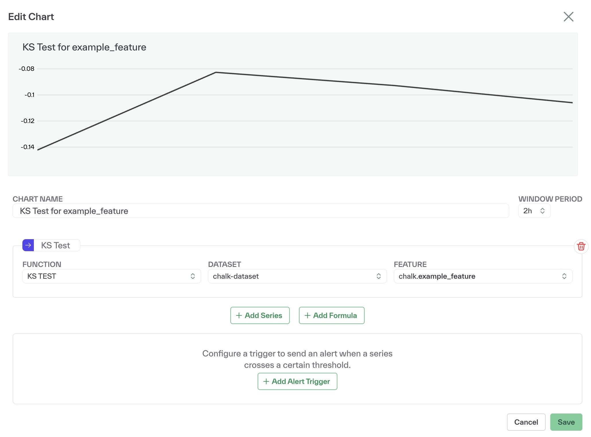
Statistical tests provide a more rigorous signal than raw summary statistics. The Kolmogorov-Smirnov (KS) test measures the maximum difference between two cumulative distribution functions — typically the training distribution and the current production distribution — to detect whether they’re drawn from the same underlying distribution. When the test statistic exceeds a critical value, it indicates statistically significant drift.
The Population Stability Index (PSI) takes a different approach: it quantifies how much a distribution has shifted relative to a reference, producing a single number that scales with drift severity. PSI scores below ~0.1 typically indicate stable distributions; scores above ~0.25 commonly signal significant drift requiring action. These are widely used rules of thumb, though appropriate thresholds vary depending on the model, use case, and how fast the data environment changes.Other commonly used methods include the Chi-Squared test for detecting shifts in categorical feature distributions, Jensen-Shannon divergence for a bounded and symmetric measure of distribution distance, and Wasserstein distance (also known as Earth Mover's Distance) for capturing the magnitude of distribution shifts in a way that accounts for the geometry of the feature space.
All these tests involve tradeoffs. More sensitive configurations detect drift earlier but generate more false positives. Less sensitive configurations reduce noise but risk missing early-stage drift. The right calibration depends on how fast your data environment changes, how costly false alarms are, and how much lead time you need before drift affects model quality.
Feature-Level Monitoring
The statistical tests above are most powerful when applied at the feature layer rather than the model output layer. As covered in the feature drift section earlier, aggregate monitoring can miss isolated feature shifts entirely — and by the time accuracy drops are measurable, the underlying drift has often been present for weeks.
In practice, feature-level monitoring means treating each feature as an independently observable signal. You track its distribution against a reference window, its freshness — the gap between when it was computed and when it's used at inference time — and its drift test statistics over time. When a feature crosses a threshold, you know exactly which part of your data pipeline to investigate before you ever see a model quality alert. That specificity is what cuts diagnosis time from days to hours.
Modern feature infrastructure makes this kind of granular monitoring practical at scale. Rather than building and maintaining separate observability tooling, teams can instrument at the feature definition level and get drift alerts, access pattern tracking, and freshness monitoring as built-in properties of how features are computed and served.
How to Handle and Mitigate Data Drift
Once drift is detected, the harder question is what to do about it. The right intervention depends on which features are affected and what the business impact is.
Root Cause Analysis with Lineage
The first step is diagnosis, and lineage is the tool that makes it possible. Data lineage — a traceable record of where each feature comes from, how it’s transformed, and which models depend on it — lets teams trace a drift signal back to its source.
Without lineage, a model accuracy drop sends teams into a debugging process that can take days: checking pipelines, reviewing upstream sources, testing hypotheses about which feature might have changed and why. With lineage, a drift alert on a specific feature includes its provenance — which upstream table it came from, which transformation produced it, which other models use it. Debugging time can drop from days to hours.
Lineage also defines the scope of impact: when a feature drifts, how many models are affected? Which downstream decisions should be reviewed? This is the kind of question that’s nearly impossible to answer reliably without a system that tracks feature dependencies end to end.
Retraining Strategies
Retraining is the most common response to data drift, and it’s often the right one — but it’s not a catch-all. There are two broad approaches: scheduled retraining, where models are retrained on a fixed cadence regardless of detected drift; and trigger-based retraining, where retraining is initiated when drift signals exceed a threshold.
Trigger-based retraining is generally more efficient but requires solid monitoring infrastructure to be reliable. Scheduled retraining is simpler to operate but may retrain models unnecessarily when there’s no meaningful drift, or fail to retrain quickly enough when drift is sudden.
The most important caution: don’t retrain without understanding why the model drifted. If a data pipeline is producing corrupted features, retraining on that pipeline’s output trains a model on corrupted data. The retrained model inherits the problem. Before triggering a retrain, confirm that the training data for the new run reflects the intended distribution — not the drifted one.
Feature Engineering Adjustments
Some drift doesn’t call for retraining at all; it calls for adjusting how features are defined. Time windows are the most common lever: if user behavior has accelerated, a 30-day rolling average may be too slow to capture meaningful signal, and shortening to a 7-day window may restore model performance without a retrain.
Other adjustments include normalization strategy changes (if the scale of raw values has shifted), decay weighting (to down-weight older data that no longer represents current behavior), and feature retirement (when a feature has become so unstable that its variance introduces more noise than signal).
Process and Governance Changes
Drift is a technical problem with an organizational dimension. Technical tooling can detect it and surface it, but responding effectively requires clear ownership: who is responsible for monitoring drift on a given feature set? Who gets alerted when a threshold is crossed? Who has authority to initiate a retrain or a feature change?
In regulated industries, the governance layer isn’t optional. The ability to demonstrate that drift was detected, investigated, and resolved within a defined timeframe — with documentation of what the model saw and when — is increasingly a compliance requirement in credit, insurance, and healthcare ML systems.
Data Drift in Real-Time ML Systems
Real-time ML systems experience drift differently than batch systems. Feedback loops are shorter. Behavioral shifts propagate faster. And unlike batch inference, where a delay of hours may be acceptable, real-time decisions require features that reflect what’s true right now — not what was true when the last batch job ran.
This creates a specific set of challenges:
- Time-aware features — rolling windows, recency-weighted aggregations, behavioral velocity metrics — are among the most predictive features in real-time systems and among the most vulnerable to drift. When user behavior accelerates or seasonal patterns shift, these features move fast.
- Freshness guarantees matter at a different level of precision. A feature that’s two hours stale may be acceptable for a weekly batch scoring job. For a fraud decision made in under 100ms at the point of transaction, a two-hour-old velocity feature can be the difference between catching fraud and missing it.
- Reproducibility is operationally critical. When a real-time model makes a decision that needs to be audited or challenged, teams need to reconstruct exactly what the model saw at that moment — which features, which values, which version. Systems that don’t capture inference-time feature snapshots make this impossible.
Often, the best answer is to compute features at inference time from live sources rather than serving pre-materialized values from a store that’s only as fresh as the last batch run. This eliminates the staleness ceiling that batch materialization creates and ensures that the features a model uses at decision time reflect current reality.
Drift Is Inevitable. Chalk Can Help.
Data drift is not a problem you solve once and move on from. It’s a permanent feature of deploying machine learning in a world that keeps changing. The question isn’t how to prevent drift — you can’t. The question is how to build systems that detect it early, diagnose it fast, and respond before it causes failures.
The teams that handle drift best share a few structural properties. They monitor at the feature layer, not just the model output layer, so they see signals before accuracy degrades. They maintain data lineage end to end, so when a feature drifts they can trace it to the source and scope the impact. They enforce freshness — their models get features that reflect current reality, not a stale cached value from a batch pipeline that ran twelve hours ago. And in real-time systems, they can reproduce exactly what a model saw at any point in time — not just for audits, but for debugging and retraining.
Chalk is built around this architecture. Mission Lane uses Chalk to power real-time credit approvals, fraud detection, and customer-facing features from a single consistent feature platform — and credits it with helping the team reduce drift and scale confidently across systems. Verisoul ships fraud detection updates 10x faster and achieves 4x more accurate detection using fresh inference-time features, with complete auditability for every decision. Across both cases, the architectural foundation is the same: feature-level observability, lineage, and freshness-aware compute, treated as system-level properties rather than afterthoughts.
“It used to take 24 hours to regenerate a training set. Now it’s under an hour. We can trust every feature in it.” — Robert Theed, Backend Tech Lead, iwoca
Modern MLOps maturity means designing systems that expect drift, not systems that assume stability. That means feature-level observability that catches distribution shifts before they cascade. It means lineage that makes root cause analysis fast. It means freshness guarantees that ensure your models are making decisions on current reality, not a snapshot from last week. And increasingly, it means extending those same properties into LLM pipelines, where prompt inputs can drift just as quietly as traditional feature distributions.
Drift is inevitable. Failures don’t have to be.
See how teams move from reactive drift detection to feature-level observability with Chalk.
[Talk to an engineer] → Get a Demo